Silver and gold are the most widely known precious metals. Apart from silver and gold, precious metals include platinum and palladium. However, what so special about silver and gold is that they have a long history of being used as money, even though they are no longer used as “money” today.
This article explores the price movement of silver and gold over the recent decades. Even though there are many ways to invest in precious metals, namely futures, contracts for differences, ETFs, owning miner stocks, or owning physical bullion, I pick the ETF way for simplicity. To track the prices of the two metals, I used ETF: GLD to track gold prices and ETF: SLV to track silver prices. This comes with an implicit assumption that the tracking errors of the ETFs are negligible, and the market close price is representative of the metal prices long term.
Correlation between gold and silver
Of late, gold price has risen by significant amount. Let’s review gold and silver price movement of the past decades.
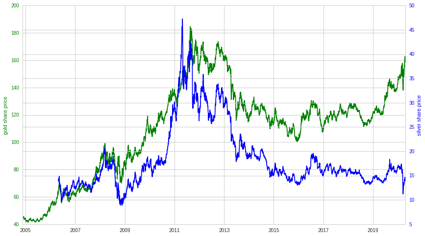
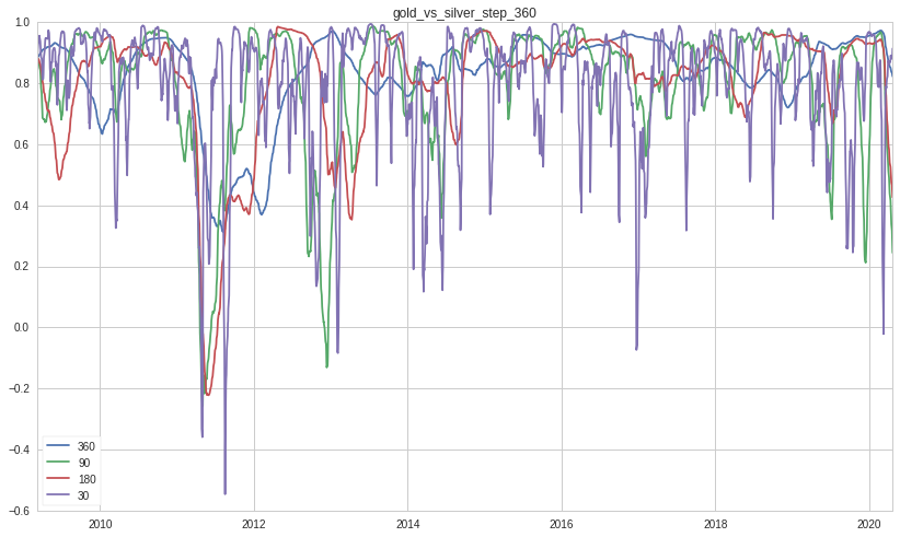
At first glance, gold and silver seem to move together or correlated. Let’s assume we buy and hold the metal and let’s calculate the return (in percentage based on the ETF price change) over different time lags(steps or holding periods) including 30, 90, 180, 360 trading days. These steps roughly translate to 1 month, 3 months, 6 months and 1 year time periods.
The correlation is calculated based on Pearson Product Moment Correlation. The windows used for the correlation calculation match the step sizes. Thus, this helps to show how the correlation varies with different holding periods of gold and silver and with different number of observations.
When we look more closely at the correlations, we can see there are periods when gold and silver largely move in tandem ( values greater than 0.7) and when the two metals move apart in opposite direction (values less than -0.1). With fewer observations (<90), the correlations oscillate significantly and widely. The oscillation reduces with more observations. As the holding period increase, the swing becomes wider also, thereby making the pattern more apparent.
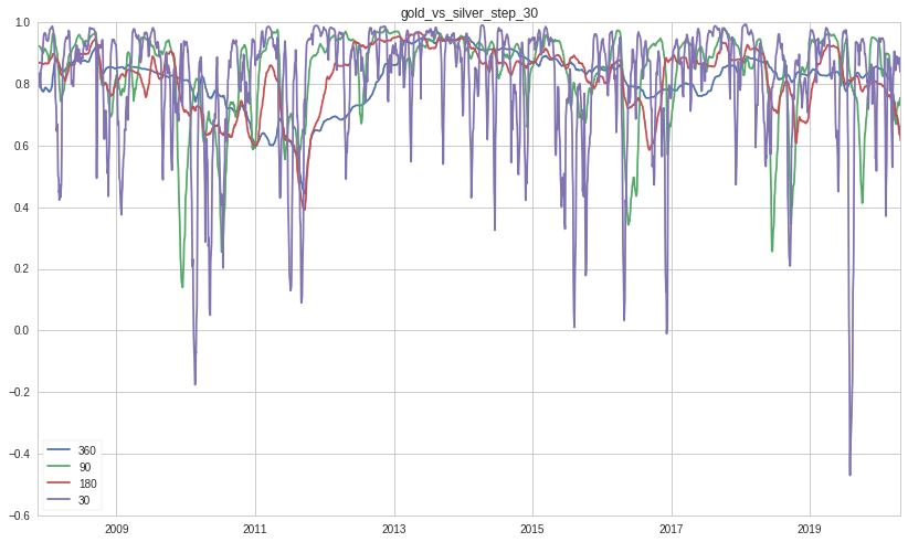
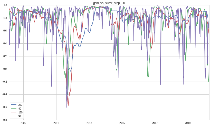
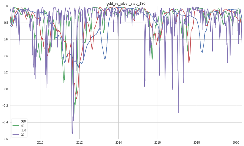
How many times the returns of gold and silver move in one direction or move in opposite direction?
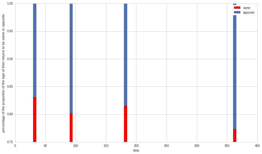
Answer: very often (shown in red)
I would like to draw several observations:
- Gold versus silver ratio cannot hold or must oscillate widely whenever the correlation becomes so unstable
- Even though gold and silver are precious metal, they can exhibit opposite behaviors as indicated by the negative correlations.
- I think after all silver has a large demand from industrial companies for manufacturing a wide array of products. Gold, on the other hand, has little industrial use (except for jewelry).
What is the distribution of returns when gold and silver move in the same direction or in the opposite direction?
Let’s take a look at situation in which gold and silver move in the same direction. Each figure show the distribution of returns (counts on y-axis; return magnitude on x-axis) (gold in green; silver in blue) with its holding period written on top. Their median is shown by a vertical line.
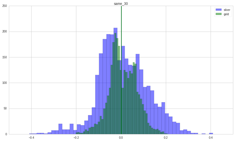
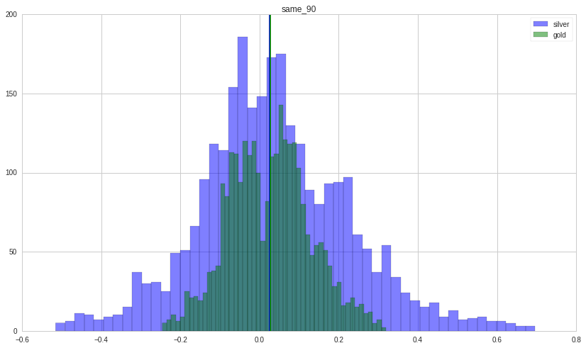
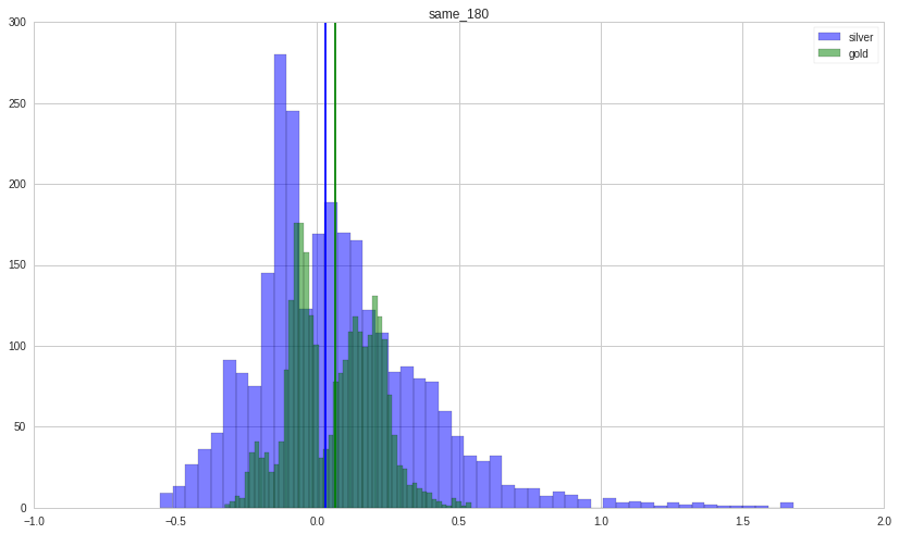
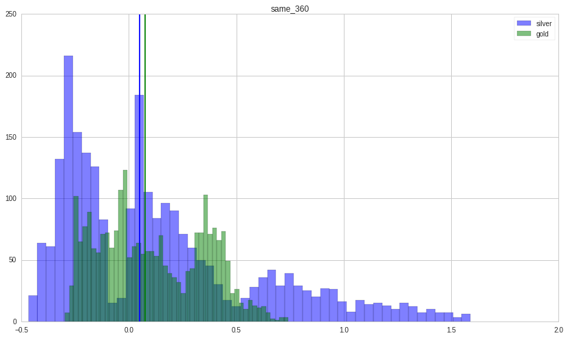
Silver is far more volatile than gold as its distribution is wider.
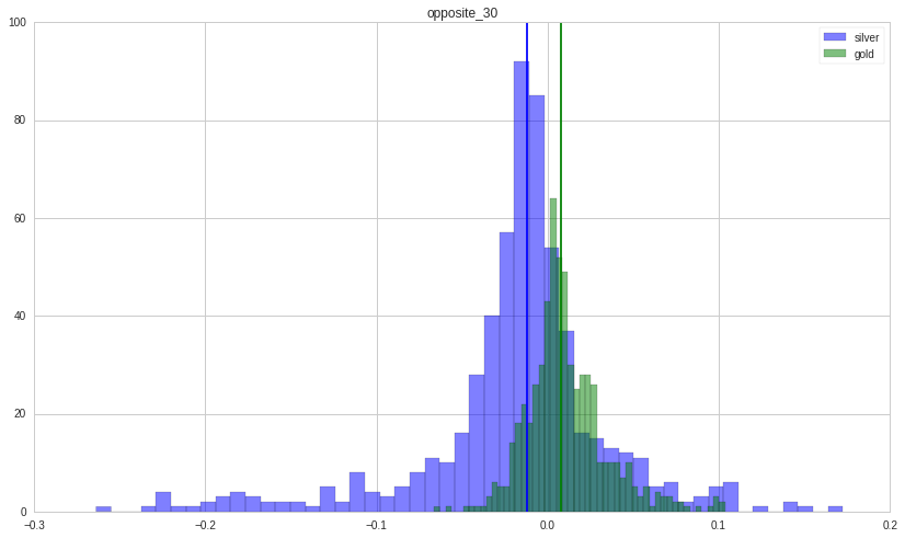
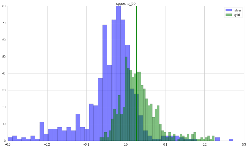
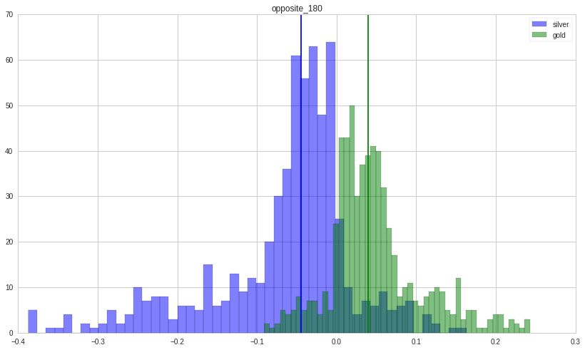
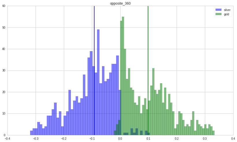
Now, we turn our attention to what happens when the returns of the two move in opposite direction. Silver tends to lose money; gold tends to make money.
Backtesting of a 90:10 gold versus silver portfolio
Quantopian algorithm backtesting platform has provided a summary of the performance.
| Annual return | 6.26% |
| Cumulative returns | 133.531% |
| Annual volatility | 19.246% |
| Sharpe ratio | 0.41 |
| Calmar ratio | 0.13 |
| Stability | 0.32 |
| Max drawdown | -48.222% |
| Omega ratio | 1.08 |
| Sortino ratio | 0.58 |
| Skew | -0.20 |
| Kurtosis | 6.85 |
| Tail ratio | 1.01 |
| Daily value at risk | -2.393% |
| Gross leverage | 1.00 |
| Daily turnover | 0.095% |
| Alpha | 0.07 |
| Beta | 0.06 |
The portfolio’s returns during different time periods or events are summarized below.
| Stress Events | mean | min | max |
|---|---|---|---|
| Lehman | -0.13% | -5.39% | 11.98% |
| US downgrade/European Debt Crisis | 0.64% | -3.85% | 3.73% |
| Fukushima | 0.35% | -0.80% | 1.65% |
| EZB IR Event | 0.06% | -0.93% | 2.25% |
| Aug07 | 0.02% | -2.44% | 1.73% |
| Mar08 | -0.49% | -4.03% | 3.19% |
| Sept08 | 0.23% | -5.39% | 11.98% |
| 2009Q1 | 0.21% | -3.94% | 4.64% |
| 2009Q2 | 0.09% | -2.94% | 3.28% |
| Flash Crash | 0.60% | -0.47% | 2.86% |
| Apr14 | -0.01% | -1.82% | 1.26% |
| Oct14 | -0.14% | -2.21% | 1.42% |
| Fall2015 | -0.01% | -1.51% | 2.11% |
| Low Volatility Bull Market | 0.01% | -7.10% | 3.64% |
| GFC Crash | 0.09% | -8.38% | 11.98% |
| Recovery | 0.07% | -6.29% | 3.73% |
| New Normal | 0.00% | -9.16% | 5.06% |

Below shows an overall summary of the performance over the entire period.

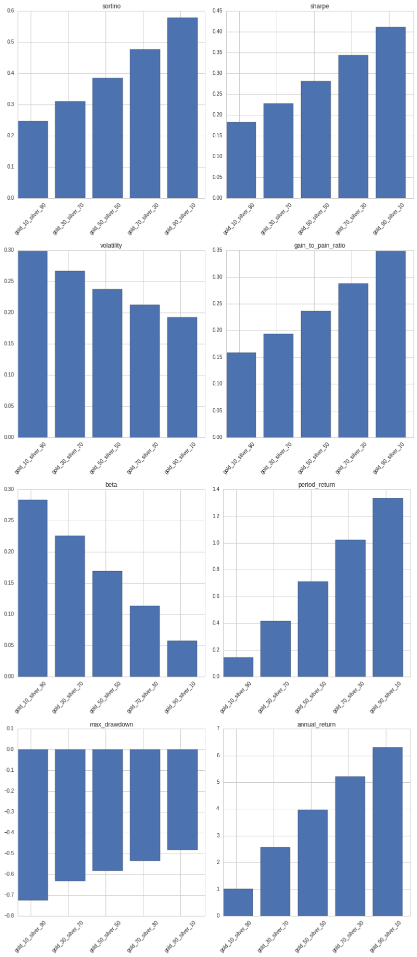
Various mix of gold and silver portfolio
From 2006-05-01 to 2020-04-23, inclusion of silver reduces returns and increases risk.
Python code
import numpy as np
import pandas as pd
import itertools
import matplotlib.pyplot as plt

def custom_change_percentage(x):
    return (x[-1] - x[0]) / x[0]


def cal_change_percentage(price_dict, ticker, step, latest):

#     print ('from {}'.format(latest))
#     print ('---%s---' %ticker)

    series = price_dict[ticker]
    series = cut_from(latest, series)
    series = series.rolling(step).apply(custom_change_percentage)
    series = series.dropna()
    return series


def cut_from(latest, series):
    mask = series.index == latest
    where = np.where(mask == True)[0][0]
    return series.iloc[where:]


def build_change_price_dict(price_dict, ticker, step, date0):

    latest = max([date0[ticker] for ticker in basket])

    for ticker in basket:

        ch_per = cal_change_percentage(price_dict, ticker, step, latest)
        price_dict2[ticker] = ch_per

    df = pd.DataFrame(price_dict2)
    return df

def cal_correlation_classes(price_dict, ticker, step, date0, basket, windows):

    correlation_dict_windows = {}

    dfs = {}

    for i, item in enumerate(itertools.combinations(basket, 2)):

        print (i, item, asset_classes[item[0]], asset_classes[item[1]])


        # build price dict, add gaps

        df = build_change_price_dict(price_dict, ticker, step, date0)
        correlation_dict = {}
        for window in windows:

            c = df[item[0]].rolling(window=window).corr(df[item[1]])


            correlation_dict[window] = c

        key = asset_classes[item[0]] + '_vs_'+ asset_classes[item[1]]
        dfs[key] = df
        correlation_dict_windows[key] = correlation_dict
    return correlation_dict_windows, dfs

def plot_correlations(correlation_dict_windows, step, period=360):

    for comparison, correlation_dict in correlation_dict_windows.items():
        plt.figure()
        plt.title(comparison + '_step_' + str(step))


        for window, value in correlation_dict.items():

#             print (value)
            L = len(value)
            if L < period:
                plt.plot(value, label=str(window))
            else:
                plt.plot(value[period:], label=str(window))

            plt.grid(b=True, which='both')


        plt.legend(loc='lower left')


price_dict2 = {}
basket = ['GLD', 'SLV']
steps = [30,90,180, 360]
windows = [ 30, 90, 180, 360]

same = {}
opp = {}

gold_dist = {'same':{},
            'opposite':{}}
silver_dist = {'same':{},
            'opposite':{}}
for step in steps:


    correlation_dict_windows, dfs = cal_correlation_classes(price_dict, ticker, step, date0, basket, windows)

    a = np.array(dfs['gold_vs_silver']['GLD'] > 0)
    b = np.array(dfs['gold_vs_silver']['SLV'] > 0)

    c = a == b
    gold_dist['same'][step] = dfs['gold_vs_silver']['GLD'][c]
    silver_dist['same'][step] = dfs['gold_vs_silver']['SLV'][c]

    c = np.sum(c) / len(c)
    d = a != b
    gold_dist['opposite'][step] = dfs['gold_vs_silver']['GLD'][d]
    silver_dist['opposite'][step] = dfs['gold_vs_silver']['SLV'][d]
    d = np.sum(d) / len(d)
    same[step] = c
    opp[step] = d

    plot_correlations(correlation_dict_windows, step)


fig, ax = plt.subplots()
# width = 0.35       # the width of the bars: can also be len(x) sequence

width = 5
same_data = [same[step] for step in steps]
opp_data = [opp[step] for step in steps]

ax.bar(steps, same_data , width,  label='same', color='r')
ax.bar(steps, opp_data, width, bottom=same_data,
       label='opposite')

ax.set_ylabel('percentage of the proportion of the sign of their returns to be same or opposite')
ax.set_xlabel('step')
ax.legend()
plt.ylim([0.75,1])

plt.show()


n_bins = 50


for situation in ['same', 'opposite']:

    for step in steps:

        plt.figure()

        plt.hist(silver_dist[situation][step].values, bins=n_bins, alpha=0.5, label='silver', color='b')
        plt.axvline(x=np.median(silver_dist[situation][step].values), color='b')
        plt.hist(gold_dist[situation][step].values, bins=n_bins, alpha=0.5, label='gold', color='g')
        plt.axvline(x=np.median(gold_dist[situation][step].values), color='g')
        plt.title(situation + '_' + str(step))
#         plt.xlim([-1,2])
        plt.legend()

plt.show()

fig, ax1 = plt.subplots()
ax1.plot(price_dict['GLD'], label='gold', color='g')
ax1.set_ylabel('gold share price', color='g')
ax1.tick_params(axis='y', labelcolor='g')

ax2 = ax1.twinx()

ax2.plot(price_dict['SLV'], label='silver', color='b')
ax2.set_ylabel('silver share price', color='b')
ax2.tick_params(axis='y', labelcolor='b')


plt.show()
