The ongoing COVID-19 pandemic has had a great impact on human society and how we treat each other. To equip ourselves with the latest knowledge on COVID-19, I have explored the use of natural language processing techniques to assist us in understanding vast volume of published research results, retrieving relevant articles, and summarizing meaning and insights from scientists around the globe.
For those who would like to take on the challenge, I encourage you to visit COVID-19-research-challenge for more detailed information.
The study of natural language processing techniques has been an ongoing effort for decades. Like the study of computer vision, it has benefited immensely from many recent advances in deep learning and artificial neural networks. However, this post uses only relatively simple and classic natural language processing techniques as these techniques are already quite good and fast at revealing topics and themes in the COVID-19 literature.
Specifically, I am going to deploy standard tools to “clean up” the texts in these articles and use Latent Dirichlet Allocation to identify underlying their common themes.
Text preprocessing
I take the meta data, which is a csv spreadsheet containing detailed information on each article from Kaggle. I keep the data consistent by removing those without titles or abstracts. In total, I am left with 46K articles.
def load_data():
    df = pd.read_csv('../covid/metadata.csv')

    mask = df['abstract'].notnull()
    mask2 =  df['title'].notnull()
    mask3 = np.all([mask, mask2], axis=0)
    df = df[['title', 'abstract', 'publish_time', 'authors']]
    df = df[mask3]

    data_list = {}
    for column in df.columns:
        data_list[column] = df[column].values.tolist()

    return data_list
The English language controls the flow and coherence of texts using stop-words which do not provide much semantic meaning on their own. Additionally, words, predominantly verbs and nouns such as singular and plural, come with different variants depending on the tense or grammatical rules. The way to undo and restore the word to its basic form is called to lemmatize a word. LancasterStemmer seems too aggressive in reducing words to their stems, and after stemming the variation of word meaning may be lost (see examples below). Finally, it is more convenient to work just with lower cases. To this end, I run the following functions to clean up the texts.
Example 1
original ['sequence', 'requirements', 'for', 'rna', 'strand', 'transfer', 'during', 'nidovirus', 'discontinuous', 'subgenomic', 'rna', 'synthesis']
no stopword ['sequence', 'requirements', 'rna', 'strand', 'transfer', 'nidovirus', 'discontinuous', 'subgenomic', 'rna', 'synthesis']
WordNetLemmatizer ['sequence', 'requirement', 'rna', 'strand', 'transfer', 'nidovirus', 'discontinuous', 'subgenomic', 'rna', 'synthesis']
LancasterStemmer ['sequ', 'requir', 'rna', 'strand', 'transf', 'nidovir', 'discontinu', 'subgenom', 'rna', 'synthes']
Example 2
original ['healthcare', 'workers', 'willingness', 'to', 'work', 'during', 'an', 'influenza', 'pandemic', 'systematic', 'review', 'and', 'meta', 'analysis']
no stopword ['healthcare', 'workers', 'willingness', 'work', 'influenza', 'pandemic', 'systematic', 'review', 'meta', 'analysis']
WordNetLemmatizer ['healthcare', 'worker', 'willingness', 'work', 'influenza', 'pandemic', 'systematic', 'review', 'meta', 'analysis']
LancasterStemmer ['healthc', 'work', 'wil', 'work', 'influenz', 'pandem', 'system', 'review', 'met', 'analys']
def lower_remove_stop_word_lemmatize(data_list, column, printout_freq=5000):
    TOKEN = re.compile(r'\b\w{2,}\b')
    # "Naive" token similar to that used by sklearn

    from nltk.corpus import stopwords
    wnl = nltk.WordNetLemmatizer()

    no_stop_word_list = []
    for i, item in enumerate(data_list[column]):
        tokens = TOKEN.findall(item)

        tokens = [token.lower() for token in tokens]

        if i % printout_freq == 0:
            print (len(tokens), tokens)
        tokens = [token for token in tokens if token not in stopwords.words('english')]
        if i % printout_freq == 0:
            print (len(tokens), tokens)
        tokens = [wnl.lemmatize(token) for token in tokens]
        if i % printout_freq == 0:
            print (len(tokens), tokens)
            print ()

        no_stop_word_list.append(tokens)

    return no_stop_word_list
A majority of the words in the texts do not occur regularly in these articles. I drop them out based on their occurrence in the entire texts of titles.
I like defaultdict because if we do not include certain words, the defaultdict would automatically throws a count value of zero without raising KeyError as in the case of “normal” dict.
I have looked at the words distribution between the titles and abstracts. From what I have seen, the words in the titles are far more informative than the words in the abstracts as far as identifying hidden topics in these documents. Being a longer passage of texts, the abstracts contain far more “less meaningful” words. This is in part due to the stop-words list not being comprehensive enough. For instance, it hasn’t filtered out words such as “also”.
    # Count word frequencies
    frequency = defaultdict(int)
    for text in data_list['title']:
        for token in text:
            frequency[token] += 1


    # Only keep words that appear more often
    processed_corpus = [[token for token in text if frequency[token] > 60] for text in data_list['abstract']]
#    pprint.pprint(processed_corpus)


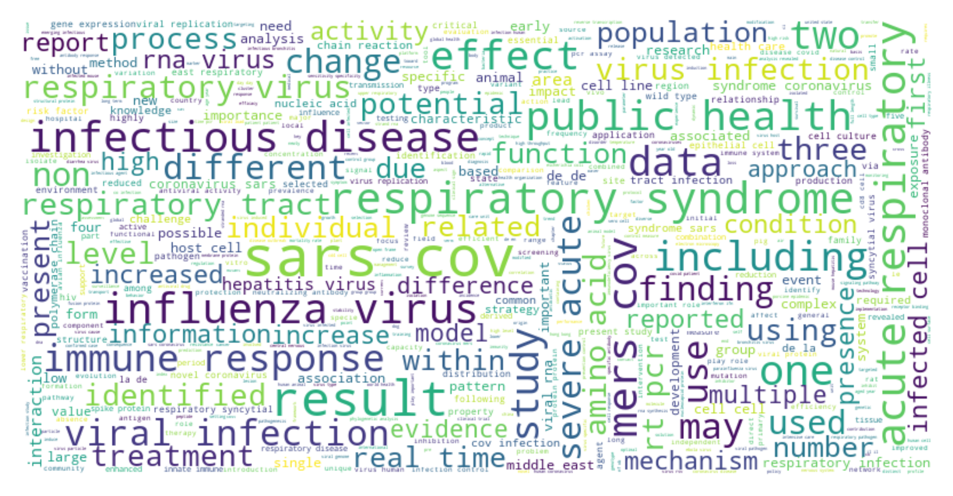
    from wordcloud import WordCloud
    text = ' '.join(flatten_list(processed_corpus))

    # Generate a word cloud image
    wordcloud = WordCloud(width=800, height=400,
                          max_font_size=50, max_words=500, background_color="white").generate(text)

    plt.figure()
    plt.imshow(wordcloud, interpolation='bilinear')
    plt.axis("off")
    plt.savefig(os.path.join(output_dir, 'processed_corpus_abstract.png'), transparent=True , dpi=400, bbox_inches='tight')
    plt.close()
How to build topic models using Gensim?
Building topic models using Gensim is very easy. Here is how I do it. Gensim is especially helpful because it puts memory usage and computational efficiency at heart. Models.LdaModel and its variants trains on the corpus incrementally, e.g. 10k at one time. This makes training feasible on less resourceful computers.
############ Gensim

    dictionary = corpora.Dictionary(processed_corpus)
    print(dictionary)


    bow_corpus = [dictionary.doc2bow(text) for text in processed_corpus]
    # train the model
    tfidf = models.TfidfModel(bow_corpus)
    corpus_tfidf = tfidf[bow_corpus]

	num_topics = 50
    topic_model = models.LdaModel(corpus_tfidf,
                                id2word=dictionary,
                                num_topics=num_topics)
#    topic_model  = models.RpModel(corpus_tfidf, num_topics=num_topics)
    # topic_model = models.HdpModel(corpus_tfidf, id2word=dictionary)
#    topic_model = models.LsiModel(corpus_tfidf,
#                                id2word=dictionary,
#                                num_topics=num_topics)  # initialize an LSI transformation
    topic_model.print_topics(num_topics)

    # both bow->tfidf and tfidf->lsi transformations are actually executed here, on the fly
    corpus_lsi = topic_model[corpus_tfidf]  # create a double wrapper over the original corpus: bow->tfidf->fold-in-lsi

    topic_words = {}

    for i in range(num_topics):
        topic_words[i] = topic_model.show_topic(i)
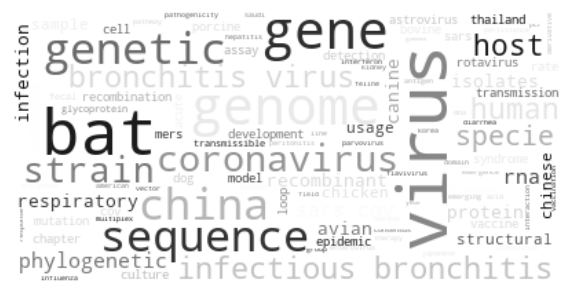
Choosing the right number of topics is not intuitive and is often a process of trial and error. For instance, 50 topics work fine in this example and I have tried a range of other numbers of topics. Since documents on different topics have different word distributions and word frequency, figuring out how to weight these words in each document is the key to identifying hidden topics amongst the documents. In essence, this is what LDA tries to do by solving for the word weights with linear algebra. The importance of words to a topic is expressed by the word weights. For example, LDA identifies topic 49th and topic 12th with the following words and their weights. I think topic 12th concerns about evolution of the virus whereas topic 49th seems to be about animal infections.
 12: [('bat', 0.06349142),
      ('specie', 0.031821612),
      ('evolution', 0.027451487),
      ('host', 0.025193721),
      ('genetics', 0.019700462),
      ('genetic', 0.017949674),
      ('virus', 0.016766567),
      ('evolutionary', 0.016061012),
      ('mutation', 0.015995547),
      ('rodent', 0.015365632)],


 49: [('dog', 0.07506799),
      ('canine', 0.05088224),
      ('2020', 0.04714561),
      ('chicken', 0.036831263),
      ('strain', 0.029606815),
      ('s1', 0.028369702),
      ('bronchitis', 0.023845471),
      ('peritonitis', 0.019557731),
      ('vaccine', 0.013181845),
      ('infectious', 0.012176985)]}
How to get a sense of what these topics are about?
Let’s take a look at what the documents say when they are likely to have come from several topics. LDA describes each document as a mixture of words taken out from an array of topics. Thus, each document naturally spreads across several topics. To really understanding what a single topic is about, the easiest way is to go through all the documents and find those that exhibit only a single topic or are heavily biased towards one topic.
To visualize these topics, I further cluster them into bigger but fewer overarching topics.
    from sklearn.cluster import MiniBatchKMeans

    n_clusters = 7
    batch_size = 3000

    kmeans = MiniBatchKMeans(n_clusters=n_clusters,
                        batch_size=batch_size,
                        verbose=0)
    counter = 0
    x = np.zeros((batch_size, num_topics), dtype=np.float16)


    # use only dominant documents for each topics
    dominant_threshold = 0.7
    for i, doc in enumerate(corpus_lsi):

        if counter % batch_size == 0 and counter > 0:
            print ('fit and reset')
            kmeans = kmeans.partial_fit(x)
            counter = 0
            x = np.zeros((batch_size, num_topics), dtype=np.float16)
        else:
            col = [item[0] for item in doc]
            v =  [item[1] for item in doc]

            # dominant document
            if max(v) > dominant_threshold:

                x[counter, col] = v
                counter = counter + 1
            # break

    print ('kmeans.cluster_centers_ {}'.format(kmeans.cluster_centers_))


    labels = defaultdict(list)
    x = np.zeros((1, num_topics), dtype=np.float16)

    for i, doc in enumerate(corpus_lsi):

        col = [item[0] for item in doc]
        v =  [item[1] for item in doc]
        x[0, col] = v
        label = kmeans.predict(x)
        labels[label[0]].append(i)

    for key, value in labels.items():
        print (key, len(value))

    # look at some documents
    max_num_samples = 300

    # randomly select some samples

    sample_set = []
    for key, values in labels.items():
        if len(values) < max_num_samples:
            s = values
        else:
            s = random.sample(values, k=max_num_samples)
        sample_set += s
    sample_set = list(set(sample_set)) # no duplicates
    ns = len(sample_set)
    print (ns, len(labels)*max_num_samples)

    X_samples_order = {i:value for i, value in enumerate(sample_set)}
    samples_X_order = {value:i for i, value in enumerate(sample_set)}


    vectors = np.zeros((ns, num_topics), dtype=np.float16)
    selected_titles = {}
    selected_abstracts = {}

    for i, (doc, abstract, title) in enumerate(zip(corpus_lsi, data_list['abstract'],
                                            data_list['title'])):


        insert_loc = samples_X_order.get(i, None)
        if insert_loc is not None:
#            print (insert_loc, i, doc, as_text)
            col = [item[0] for item in doc]
            v =  [item[1] for item in doc]
            vectors[insert_loc, col] = v
            selected_titles[i] = title
            selected_abstracts[i] = abstract

    samples_labels = kmeans.predict(vectors)

    # show the clusters of topics
    num_dimensions = 2

    tsne = TSNE(n_components=num_dimensions)
    lower_vectors = tsne.fit_transform(vectors)

    import matplotlib

    cmap = matplotlib.cm.get_cmap('tab20b')
    vmin = min(samples_labels)
    vmax = max(samples_labels)

    plt.figure(figsize=(12, 12))
    colors = ['black', 'purple', 'blue', 'green', 'orange','red','yellow']
    colormap_names = ['Greys', 'Purples', 'Blues', 'Greens', 'Oranges', 'Reds', 'spring']
    for i in range(n_clusters):
        where = samples_labels == i

        plt.scatter(lower_vectors[where,0],
                    lower_vectors[where,1], c=colors[i])
    # plt.colorbar()
    plt.axis("off")
    plt.savefig(os.path.join(output_dir, 'tsne_dominant_documents_topics.png'), transparent=True , dpi=400, bbox_inches='tight')
    plt.show()
MiniBatchKMeans has been very useful because it allows incremental fitting of the document vectors, a method that drains less computational resources but achieves similar results to KMeans.
TSNE is used to visualize the topic space in 2D.
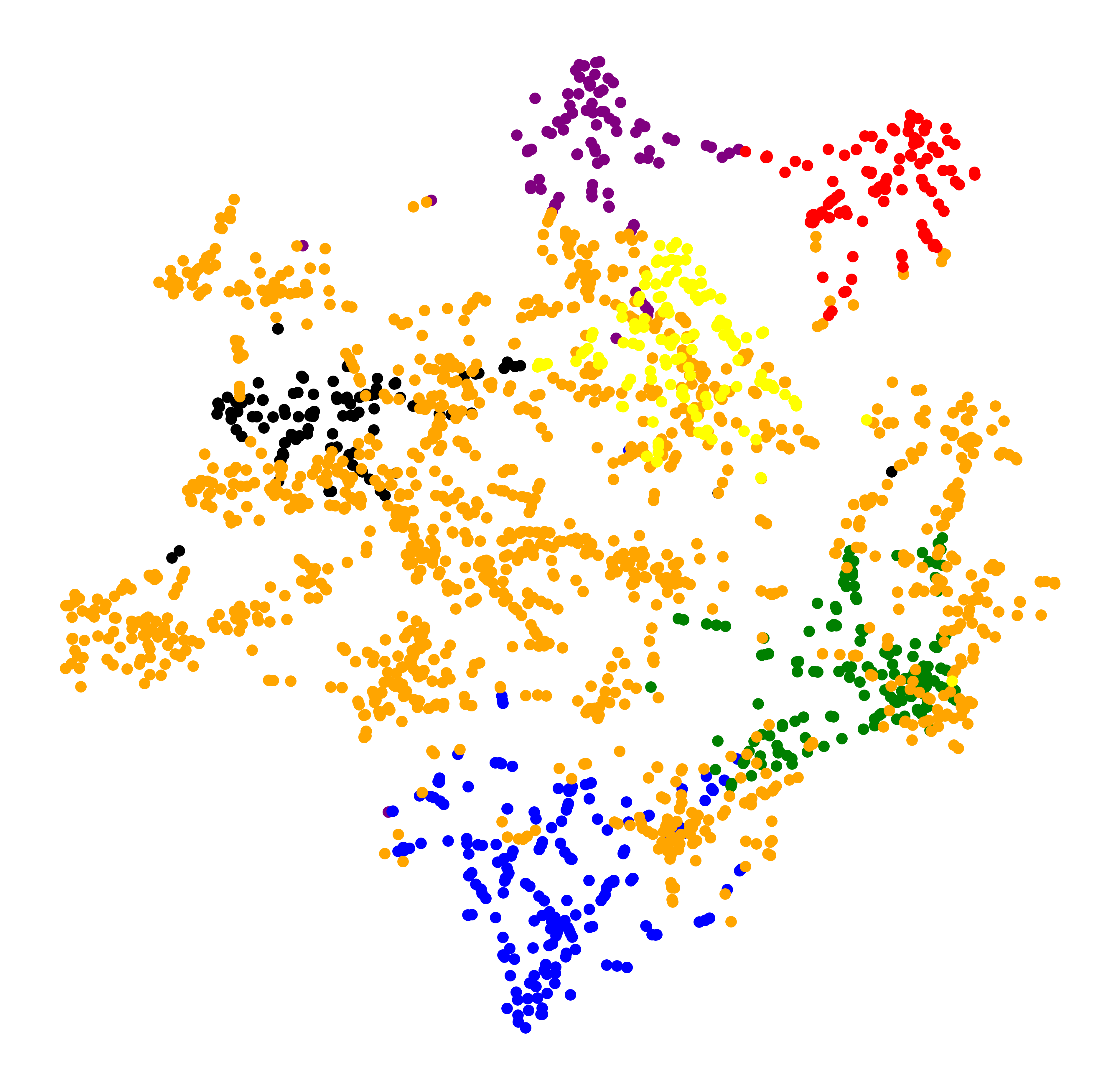
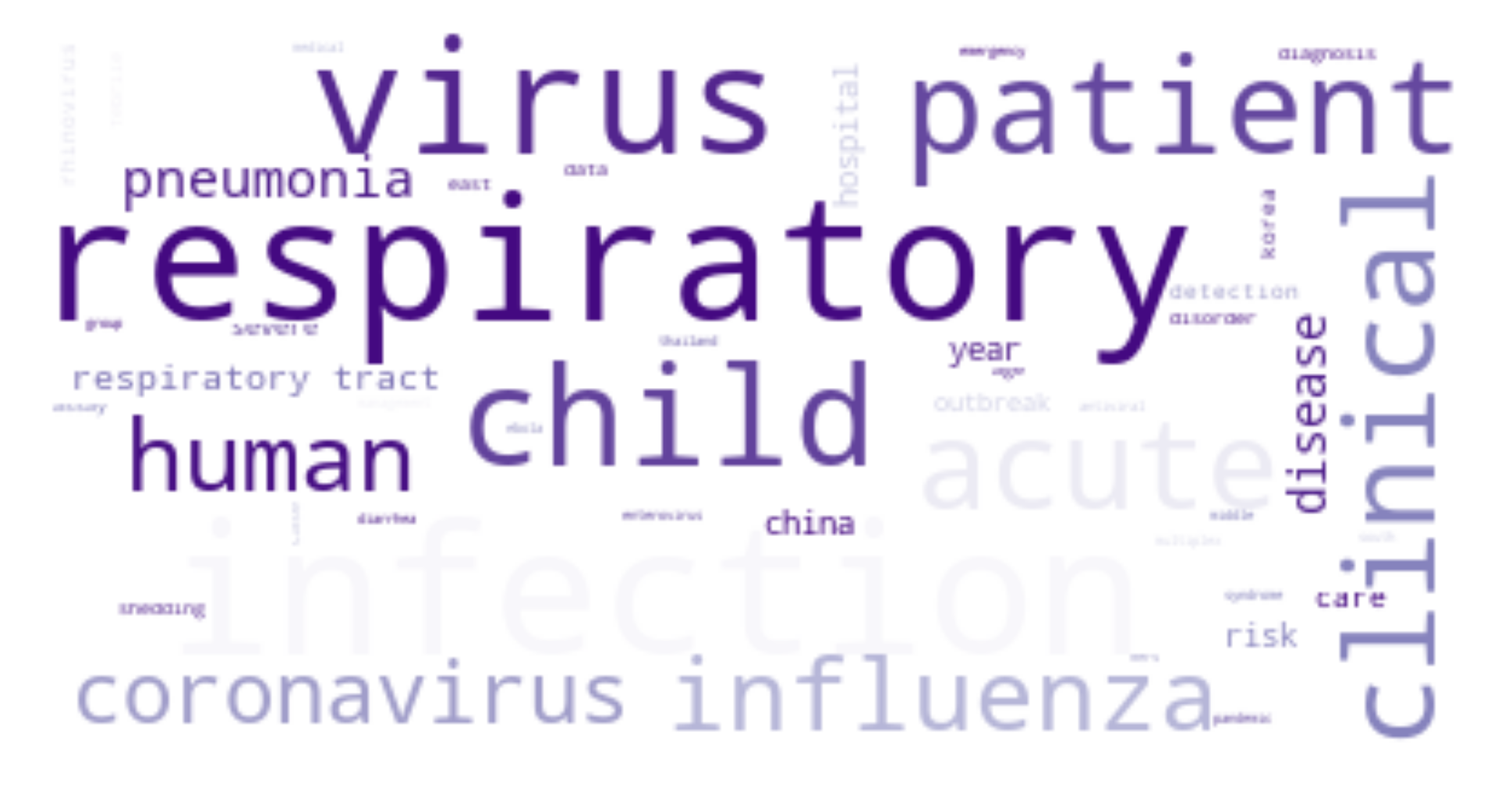
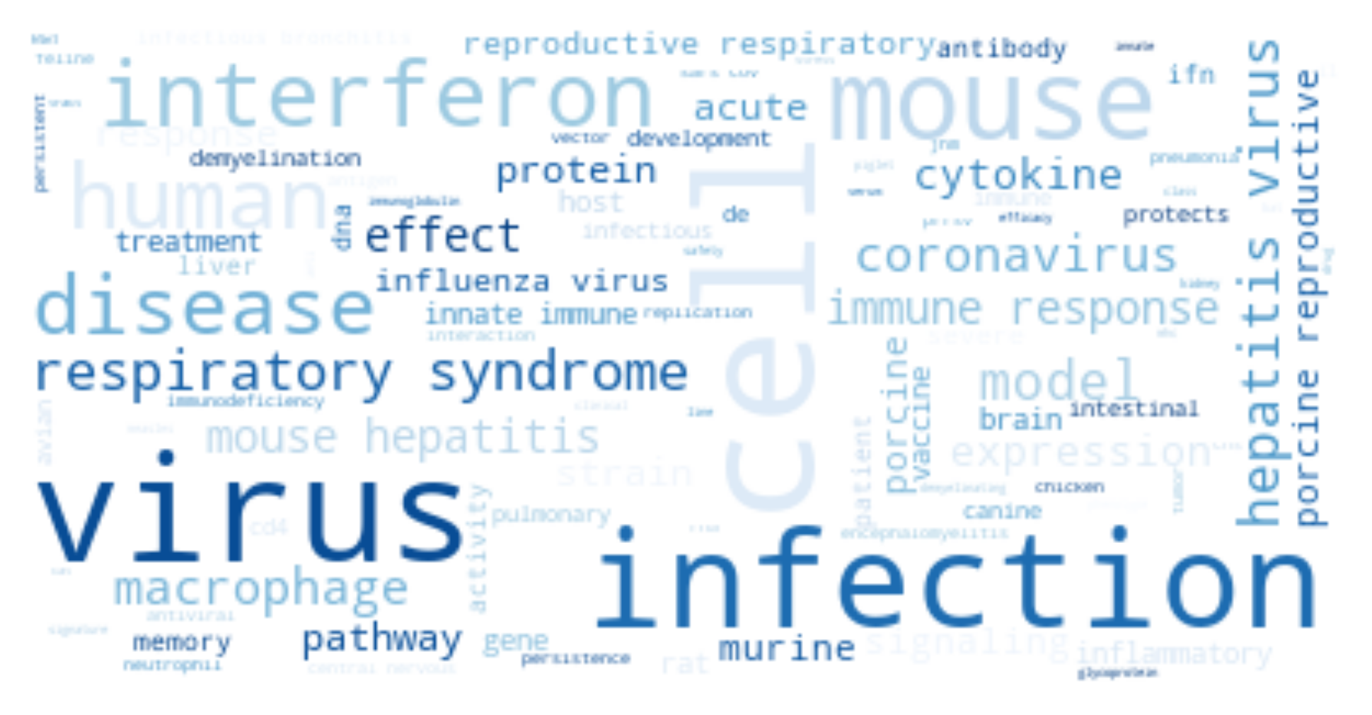
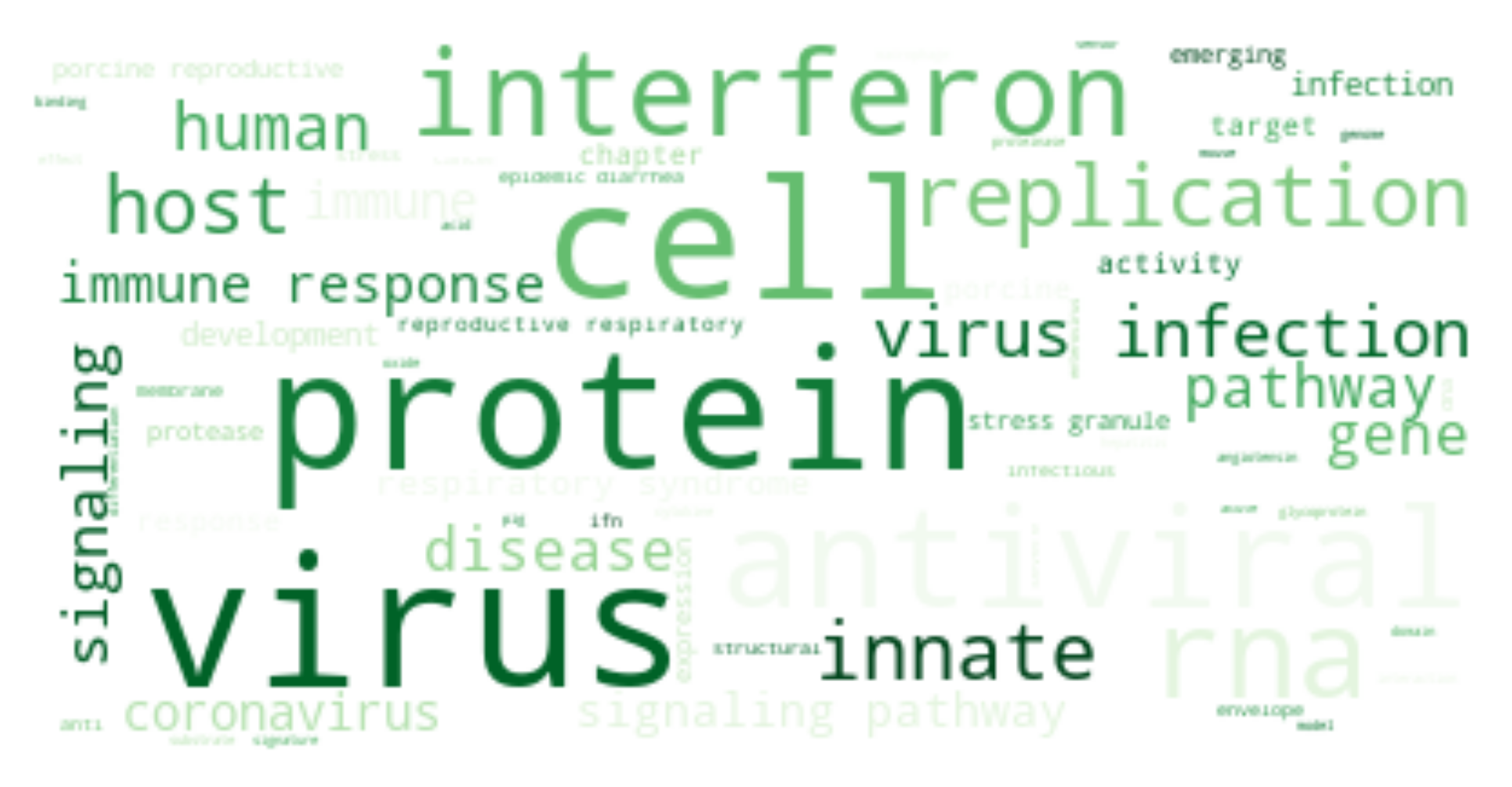
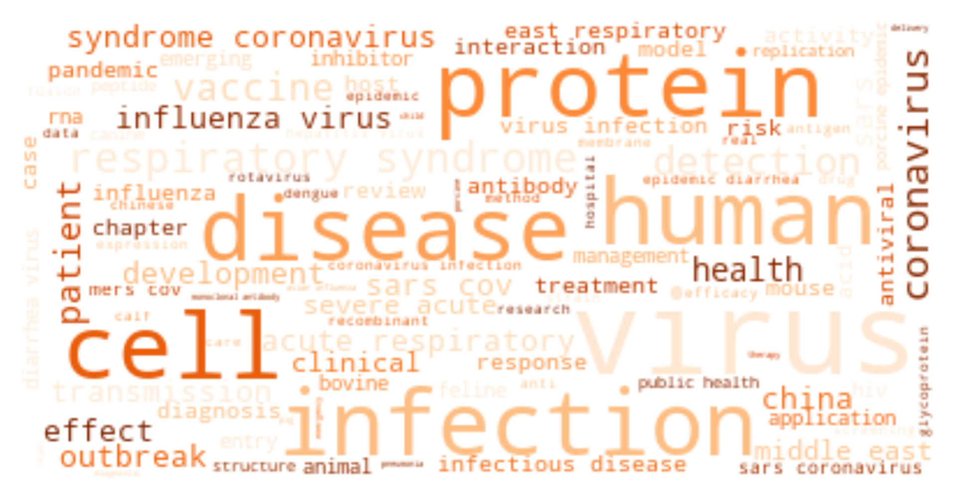
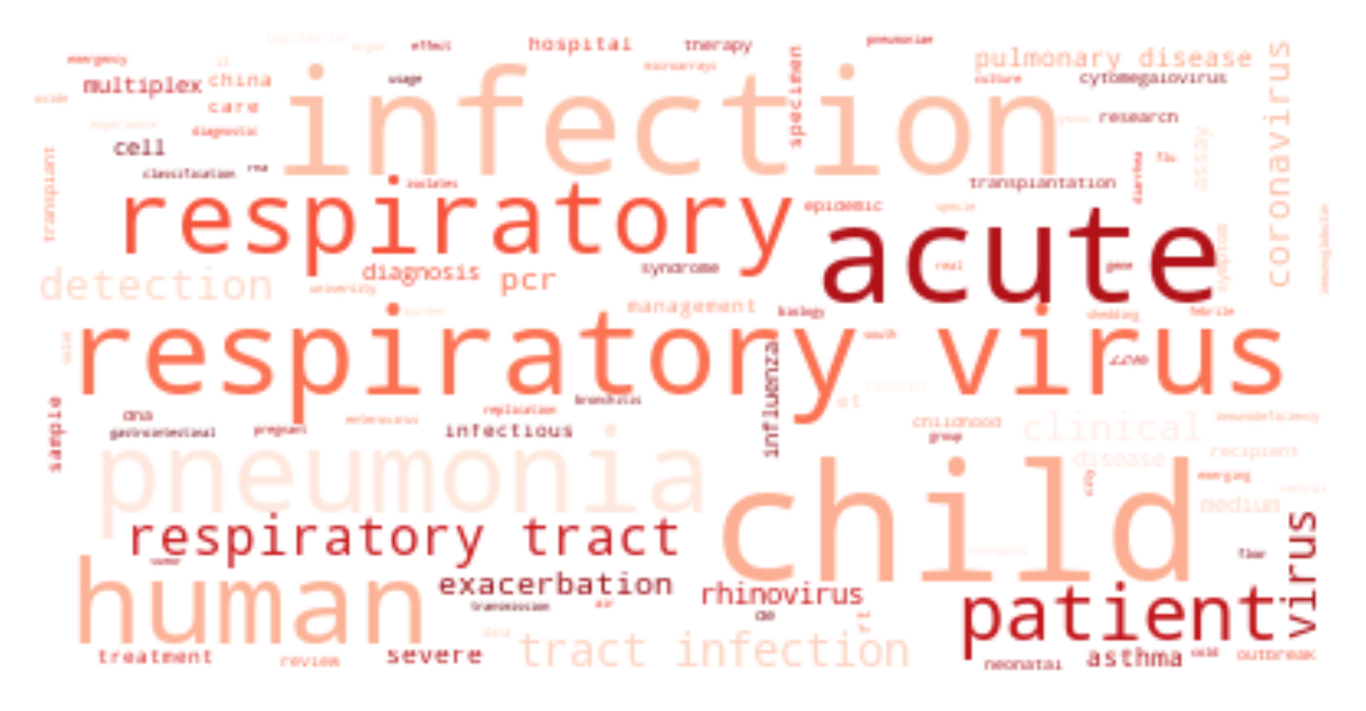
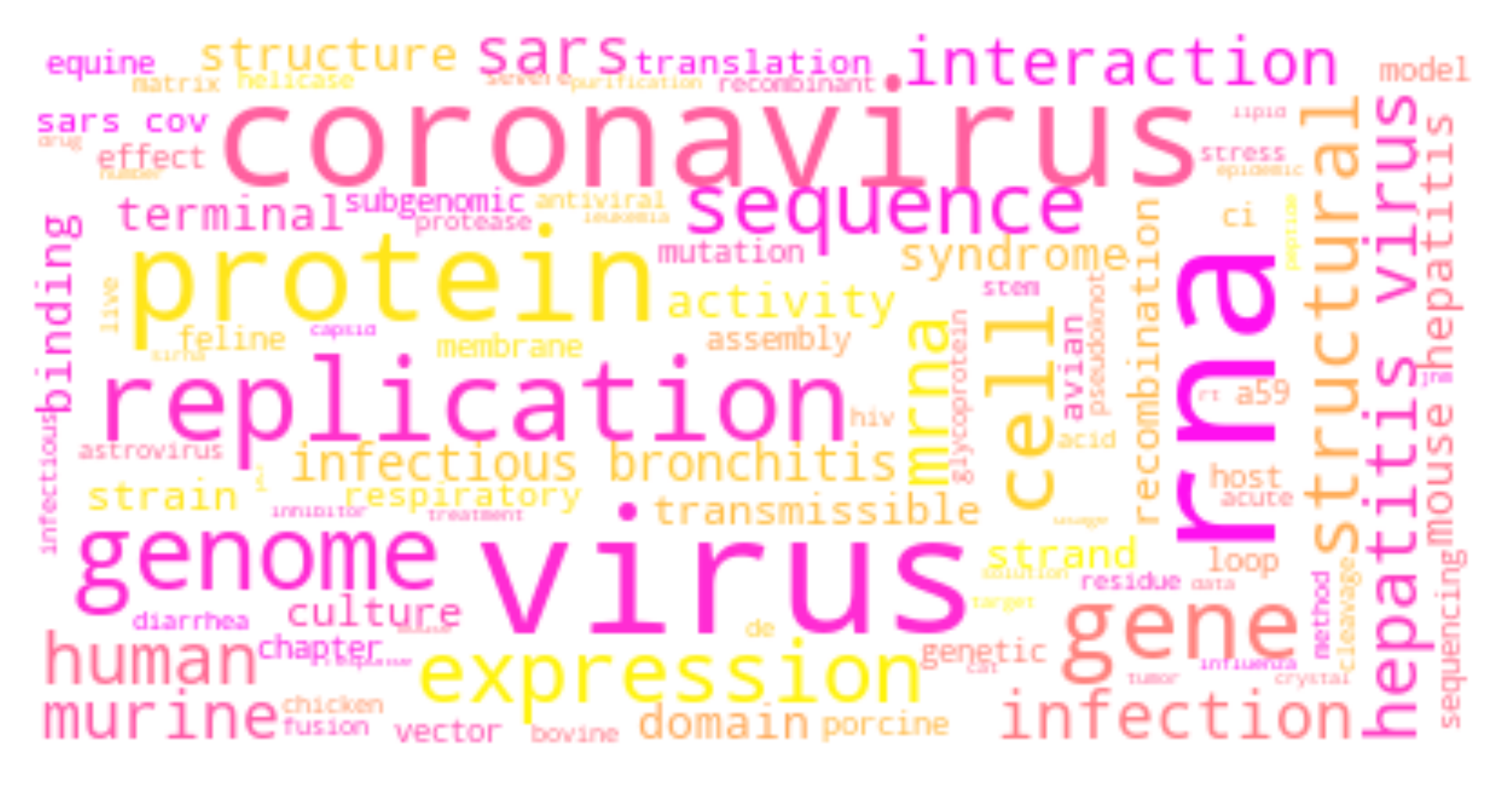
For each cluster, I have drawn its wordcloud (sharing the same color theme).
