Introduction
I have explored interesting and beautiful patterns with the help of mathematics. Here I share with you some of the famous temporal and spatial patterns we could derive using equations. The patterns include Chaos from Lorenz system, Randomness (a lack of pattern itself) from a random walk model, Regress to Mean, Folding from Henon Group. Because of their temporal and spatial nature, I present them to you in videos.
Prerequisite
- Install Anaconda 3
- Install Mayavi and its dependencies
Lorenz System
Lorenz system and its attractors are one of the most famous examples of Chaos on the Internet. We can find the basic background information from Wikipedia. To avoid repetition, I ought not to re-write what’s on Wikipedia and ought to show you my code that draws the “butterfly” pattern. It is very important to emphasize that its solution ONLY becomes chaotic with specific initial conditions and coefficients.
Load libraries and modules
import time
import numpy as np
from scipy.integrate import solve_ivp
import matplotlib.pyplot as plt
from mpl_toolkits.mplot3d import Axes3D
Initial conditions and coefficients used in this article.
sigma, beta, rho = 10, 2.667, 28
y0 = [0,1,1.05] #initial position
Lorenz equations; the integration of the ODEs is performed by a numerical method (Explicit Runge-Kutta method of order 5) implemented in Scipy.
# time steps
tmax,n = 100, int(5e4)

def lorenz(t, X, sigma, beta, rho):
    u,v,w = X
    up = -sigma*(u-v)
    vp = rho*u - v -u*w
    wp = -beta*w + u*v
    return up, vp, wp

t = np.linspace(0, tmax, n)

start_time = time.time()
soln = solve_ivp(lorenz, (0, tmax), y0, args=(sigma, beta, rho), dense_output=True)
x,y,z = soln.sol(t)
print ('integration taken {}'.format(time.time() - start_time))
Visualization (3D)
from mayavi import mlab
fig=mlab.figure(1, bgcolor=(0, 0, 0), size=(16*60, 16*60))
line = mlab.plot3d(x,y,z,t, line_width = 10)
scatter = mlab.points3d(x[0], y[0], z[0], scale_factor = 5, mode='arrow')

@mlab.animate(delay=10)
def anim():
    for ni, (i,j,k) in enumerate(zip(x,y,z)):
        scatter.mlab_source.set(x=i,y=j,z=k)
        filename = str(ni) + '.png'
        mlab.savefig(filename=filename)

        yield

fig = mlab.gcf()
fig.scene.reset_zoom()
view = (-25.53261881918745, 127.13833071761842, 154.30086011420792, np.array([ 0.70852142,  1.38596485, 24.30126513]))
mlab.view(*view)
anim()
mlab.show()
Visualization (2D)
fig, axes = plt.subplots(3,1, sharex=True, sharey=True)
for a, data, name in zip(axes, [x,y,z], ['x', 'y', 'z']):
    a.plot(t,data)
    a.set_title(name)
plt.show()


import pandas as pd

df = pd.DataFrame.from_dict({'x':x,
                             'y':y,
                             'z':z})


fig, axes = plt.subplots(3,1, sharex=True, sharey=False)
for a, data, name in zip(axes, [x,y,z], ['x', 'y', 'z']):
    a.plot(t,data,color='blue')
    a.set_title(name)
    a.grid()


for color, window in zip(['red', 'orange', 'green', 'yellow', 'black'],
                  [200, 400, 600, 800, 1200]):
    avg = df.rolling(window).mean()
    for a, name in zip(axes,  ['x', 'y', 'z']):
        a.plot(t, avg[name], color=color, label=str(window))


# plt.grid()
plt.legend()
plt.show()
Figures and Videos

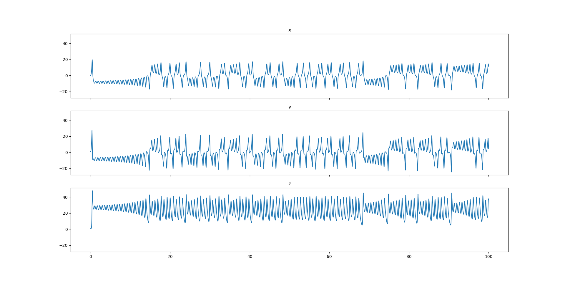
The oscillation of the positions appears quite random and chaotic if we rely only these 2D plots. However, we can clearly identify interesting motions when we create a 3D video.
The arrow denotes an instantaneous position (x,y,z,t). The line denotes the arrow’s trajectory, and its color depicts the time elapsed. In the video, we can see the arrow hops between the left and right wings while orbiting the respective centers.

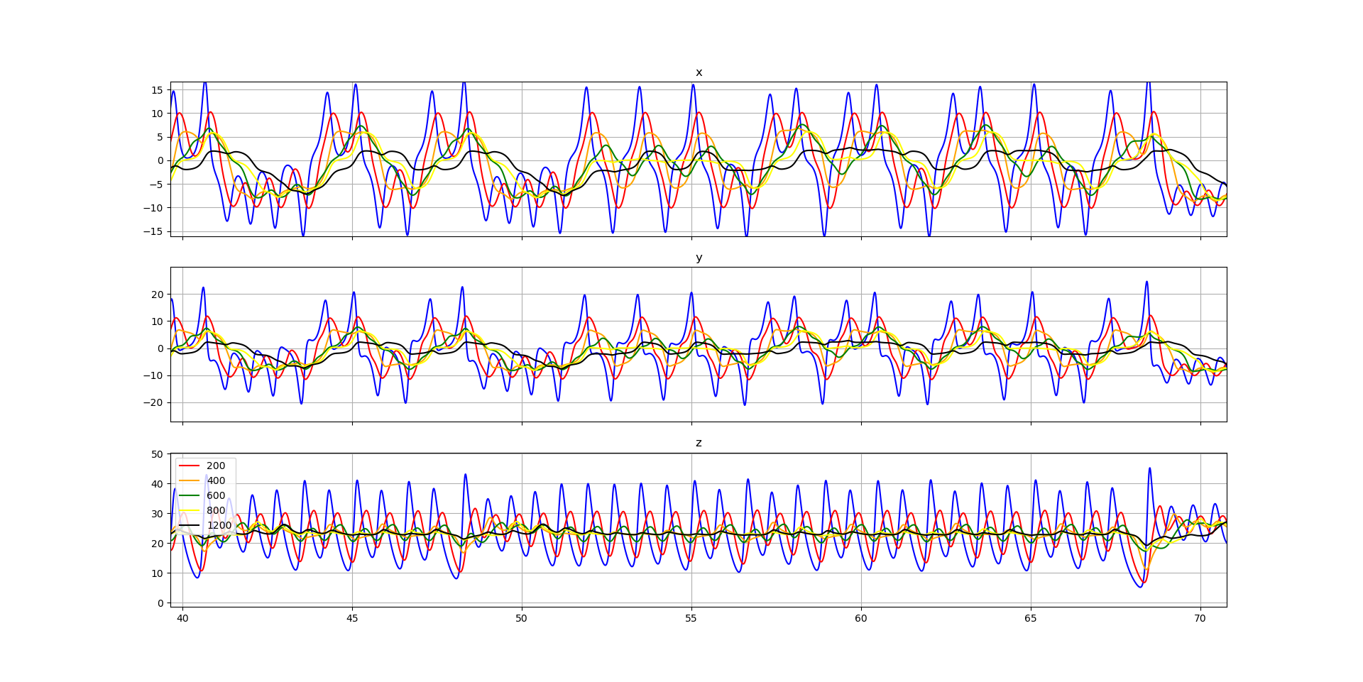
Regress to Mean is an interesting concept to explore a bit further. I added a series of moving averages (non-blue lines) of each individual spatial component (x,y,z) (in blue). When we follow the averages, the position appears to drift away from and then pull back towards the averages over time.
Henon Group
Apart from Chaos, Henon group is interesting, for they concern with the concept of folding. I take the equations and background materials from mathworld. The tutorial shows that the pattern mirrors itself as if we have just drawn the pattern on a piece of paper and then folded the paper in half. Thus, we have a pair. However, the tutorial only explains a 2D Henon group. So I create a 3D Henon group by duplicating its y onto z.
def get_next_step(c0,a=0.2,b=0.9991):
    x,y,z = c0
    x1 = y + 1 - a*x*x
    y1 = b*x
    z1 = y
    return np.array((x1, y1, z1))

c0 = [0,0,0]

num_steps = 10000
t = np.linspace(0,1,num_steps)
results = np.zeros((num_steps, 3))

for i in range(num_steps):
    if i == 0:
        results[i,:] = get_next_step(c0)
    else:
        results[i,:] = get_next_step(results[i-1,:])
The pair is shown in the video. Each dot represents a spatial location. Its colour denotes the time elapsed. The spinning effect is added to enhance the feeling of the sense of universe and its galaxies.
@mlab.animate(delay=10)
def anim():

    for angle in np.linspace(0,360, 720):
        mlab.roll(angle)
        filename = str(angle) + '.png'
        mlab.savefig(filename=filename)
        # print (mlab.view())
        # mlab.pitch(angle)
        # mlab.yaw(angle)
        yield


view = (165.62351678494917, 33.92495926342261, 29.14422638311501, np.array([0.04513454, 0.04509211, 0.04504395]))
fig=mlab.figure(1, bgcolor=(0, 0, 0), size=(16*60, 16*60))
s = mlab.points3d(results[:,0],results[:,1],results[:,2], t, scale_factor=0.1)
mlab.view(*view)
anim()
mlab.show()
Random Walk
So far, we have explored two deterministic systems, namely Lorenz system and Henon Group. We turn to the exact opposite: pure Randomness. I model Randomness using a popular random walk model. Unlike Lorenz system and Henon group that offer a deterministic numerical solution, random walk is 100% stochastic and therefore indeterminable.
num_steps = 10000
delta = np.random.rand(num_steps, 3) - 0.5 # velocity ranges between +- 0.5
# initial starting position is zero
positions = np.cumsum(delta, 0) # a quick way to integrate the velocity to get positions

x,y,z = positions[:,0], positions[:,1], positions[:,2]
t = np.linspace(0,1,num_steps)

fig, axes = plt.subplots(3,1, sharex=True, sharey=True)
for a, data, name in zip(axes, [x,y,z], ['x', 'y', 'z']):
    a.plot(t,data)
    a.set_title(name)
plt.show()
Figures and Videos
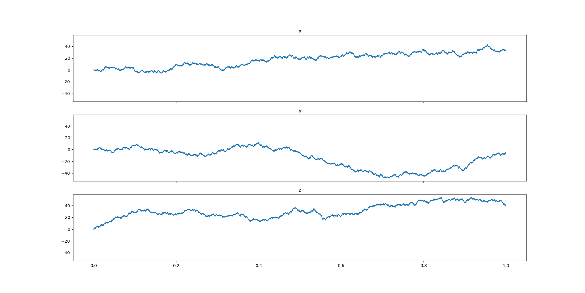
What I am showing you here is just one possible solution out of infinite solutions.

The trajectory appears to be trending somewhere in 3D. It therefore fools me into believing that I can predict its final resting place. Once again, let’s watch it in motion.
The arrow denotes an instantaneous position (x,y,z,t). The line denotes the arrow’s trajectory, and its color depicts the time elapsed. In the video, we can see the arrow zigzag. However, one must not be fooled that it is going anywhere! (as an aside, the arrow in fact follows the smoothed trajectory (smoothing window size = 100), instead of the raw trajectory. This improves the visual appeal as it reduces the arrow’s acceleration)

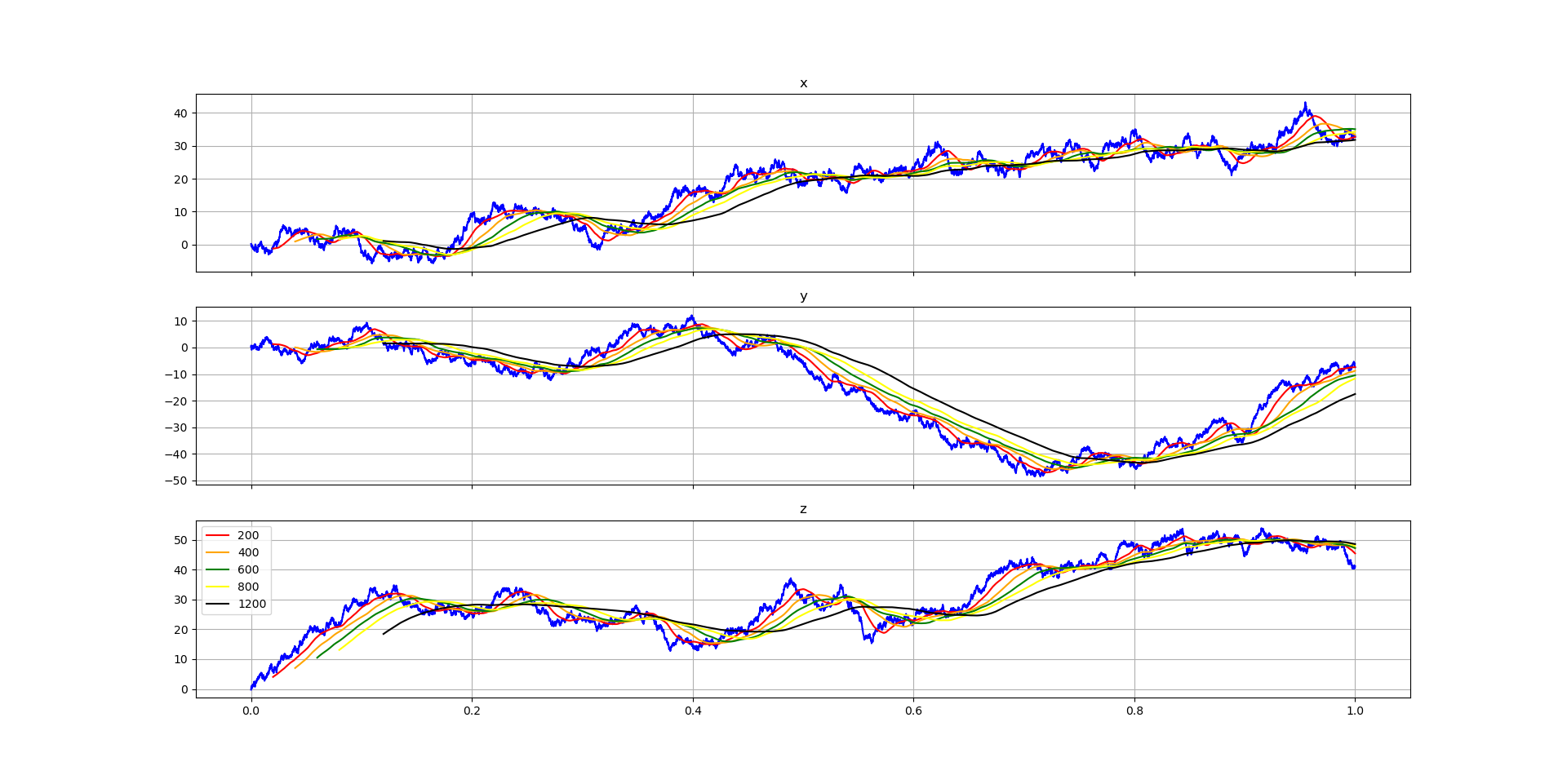
Regress to mean is robustly at work; it appears that the blue line spends about equal amount of time above and below the series of averages lines.
import pandas as pd

df = pd.DataFrame.from_dict({'x':x,
                              'y':y,
                              'z':z})


fig, axes = plt.subplots(3,1, sharex=True, sharey=False)
for a, data, name in zip(axes, [x,y,z], ['x', 'y', 'z']):
    a.plot(t,data,color='blue')
    a.set_title(name)
    a.grid()


for color, window in zip(['red', 'orange', 'green', 'yellow', 'black'],
                  [200, 400, 600, 800, 1200]):
    avg = df.rolling(window).mean()
    for a, name in zip(axes,  ['x', 'y', 'z']):
        a.plot(t, avg[name], color=color, label=str(window))


# plt.grid()
plt.legend()
plt.show()


from mayavi import mlab
fig=mlab.figure(1, bgcolor=(0, 0, 0), size=(16*60, 16*60))
line = mlab.plot3d(x,y,z,t, line_width = 30)

# only watch the smooth motion
avg = df.rolling(100).mean()
avg = avg.dropna()
avg = avg.values
x,y,z = avg[:,0], avg[:,1], avg[:,2]
scatter = mlab.points3d(x[0], y[0], z[0], scale_factor =4, mode='arrow')

@mlab.animate(delay=10)
def anim():
    degree = 0
    for ni, (i,j,k) in enumerate(zip(x,y,z)):
        scatter.mlab_source.set(x=i,y=j,z=k)
        mlab.roll(degree)
        degree += (360 / len(avg))
        filename = str(ni) + '.png'
        mlab.savefig(filename=filename)

        yield
fig = mlab.gcf()
fig.scene.reset_zoom()
anim()
mlab.show()
Conclusion
I hope you like seeing patterns that appear random but in fact deterministic as well as patterns that appear deterministic but in fact purely random.
Create Video from Image Series
This handy script builds video by stitching images (in chronological order).
import os
import imageio

files = {float(key.rstrip('.png')): key for key in os.listdir('.') if '.png' in key and 'Figure' not in key}


writer = imageio.get_writer('RandomWalk.mp4', fps=30)
for key in sorted(files.keys()): #make sure all images are in sequential order !
    file = files[key]
    writer.append_data(imageio.imread(file))

writer.close()
